These notes and tables are largely based on Pretrained Transformers for Text Ranking: BERT and Beyond.

There might be mistakes in this article. Seek the original source (see above) for confirmation if something doesn't make sense. email me if you find any mistakes so I can fix them.

In short, there are 3 different types of Transformer IR models:

1. Sparse Methods

2. Dense Methods:

3. Hybrid Methods: Combines Sparse and Dense

We will discuss each and compare them.

1. Sparse Methods

Sparse retrieval methods work as follows:

1. TF-IDF, Bag-of-Words (BoWs) exact-matching, or BM25 are used to retrieve k documents

2. The k documents are then reranked using a more sophisticated model, such as a neural network

Part (b) is of special interest.  We shall explain some models that are used for this purpose. For this purpose, we will use the following notation:

• Let docs = all documents

• Let first-docs = documents retrieved in the first stage by BM25 (“first” refers to first stage)
  • Given sentence $S = [w_1, w_2, …, w_t]$ consisting of words $w_i$, $BERT(S)[w_i]$ refers to the embedding created for $w_i$ when running through BERT. That is $BERT(S) = [BERT(S)[w_1], BERT(S)[w_2, …, BERT(S)[w_t]]$

1.1. monoBERT

We start with a pre-trained checkpoint of BERT.

Given query q, BM25 to generate first-docs. Then:

For d in first-docs:
	S = [CLS]  d  [SEP]  q [SEP]
	emb = BERT(S)[CLS]
	score  = FullyConnectedLayer(emb)

That is, we put the query and each document in a template and pass it to pert and use the embedding BERT generates for the CLS token. CLS refers to the classification task and BERT treats it as a special token to perform a classification task. Note that emb is a vector. Hence, we use a fully-connected layer to estimate the probability P(d is relevant to q); above this is referred to as the score.

The fully connected layer and BERT are trained end-to-end using the cross-entropy loss. In this way we fine-tune the pre-trained BERT model we started with.

CAL Pseudocode

In the setting of CAL, the query is regenerated at each timestep according to the previously identified relevant documents. So, at test time, our pseudocode will be:

# refine_query can have multple implementation; one such implementation is included below
def refine_query(q, d) {
	q = q + d
	trim q to 256 tokens
}


def get_doc(q) {
	For d in get_docs_logistic_regression(docs):
		S = [CLS]  d  [SEP]  q [SEP]
		emb = BERT(S)[CLS]
		score  = FullyConnectedLayer(emb)
	return d with highest score
}

query = get_query_from_user()
while (get_doc(query) returns a document) {
	let d = get_doc(query)
	show d to user
	if user_clicks_rel(d):
		refine_query(q, d)
		remove d from docs
}

This pseudo-code generalizes to other methods discussed below by simply changing the get_doc subroutine.

1.2. duoBERT

Similar to monoBERT, but it measures the probability of document $d_i$ being more relevant to $q$ than $d_j$. As such, the algorithm is slightly different

For d_i d_j in first-docs:
	S = [CLS] q [SEP] d_i [SEP] d_j [SEP]
	emb = BERT(S)[CLS]
	p_i_j  = FullyConnectedLayer(emb)

Then the score for each document $d_i$ is calculated based on all $p_{i,j}$ using either a sum/min/max function, e.g. $s_i = \max_{j}(p_{i,j})$, or by counting the number of occurrences where $p_{i,j} > 0.5$.

Note: For efficiency purposes duoBERT is usually used as a second reranker after monoBERT. That is, we usually rank with BM25, then rerank with monoBERT and then use duoBERT to rerank the top k documents from monoBERT. duoBERT usually have a modest improvement over simply using monoBERT.

1.3. monoT5

Similar to monoBERT but T5 is used instead of BERT.

For d in first-docs:
	S = query: q doc: d relevant:
	out = T5(S)
	score = softmax(out[true], out[false])

monoT5 performs better than monoBERT and duoBERT.

1.4. duoT5

Similar to duoBERT but uses T5 instead of BERT:

For d_i d_j in first-docs:
	S = query: q doc1: d_i doc2: doc_j relevant:
	out = T5(S)
	score = softmax(out[true], out[false])

Note that here "relevant" refers to $d_i$ being more relevant than $d_j$

2. Dense Methods

Dense methods use representation learning. In particular, they work as follows:

For our setting, both $\eta_q$ and $\eta_d$ are transformer-based neural networks. In practice, $\eta_q$ and $\eta_d$ can be the same model.

Also, in theory $\phi$ can be any function such as another transformer-based neural network. But, this defeats the purpose of dense retrieval since 1) neural network models are not fast to compute 2) it would be equivalent to monoBERT.

In practice, $\phi$ is a fast-to-compute function, such as the inner-product.

Hence, we compute the score for document $d_i$ as follows: $s_i = \phi(\eta_q(q), \eta_d(d_i)) = \langle\eta_q(q), \eta_d(d_i)\rangle$

Ranking is done based on this score.

It is also common to write $\eta_i = \eta_d(d_i)$ and $\eta_q = \eta_q(q)$

2.1. DPR

DPR (Dense Passage Retrieval) is one of the most well-known dense retrieval models.

DPR calculates the score as follows: $s_i = \langle BERT(d_i)[CLS], BERT(q)[CLS] \rangle$

Note that the two BERT models here do NOT share weights, so they are fine-tuned separately.

The model is trained using a dataset where each datapoint consists of a query, a positive document and $n$ negative documents. That is each datapoint is as follow: $[q_i, d_i^+, d_{i,1}^-, ..., d_{i,n}^-]$. In practice, choosing the negative samples for each query has a large impact on the effectiveness of the model. Although simple models such as BM25 can be used, they do not yield the best results. There are other approaches proposed such as ANN (Approximate Nearest Neighbour) search to find non-relavant documents that are ranked high by the model. This creates a learning-loop so the model can learn from its mistakes.

2.2. ANCE

ANCE (Approximate Nearest Neighbor Negative Contrastive Estimation) works as follows:

ANCE calculates the score as follows: $s_i = \langle RoBERTa(d_i)[CLS], RoBERTa(q)[CLS] \rangle$

Unlike DPR, ANCE uses RoBERTa. Also, in contrast to DPR, the two RoBERTa models in ANCE share weights; that is they are the same model.

Datapoints to train ANCE are similar to that of DPR and the negative examples are chosen using a ANN approach.

Sparse vs. Dense

Dense retrieval methods, such as the ones explained above underperform (with respect to metrics such as MRR) compared to multi-stage sparse methods discussed previously (e.g. using BM25 to get a first stage ranking and using monoBERT/monoT5 to rerank the documents). However, at test time, these dense methods are much faster than the sparse methods discussed previously since the embedding of the documents can be pre-computed in parallel and stored before the test time. As such, these dense methods only need to embed the query and compute the efficient similarity metric between the embedding and each of the already-stored document embeddings.

PreTTR

PreTTR (Precomputing Transformer Term Representations) is similar to a monoBERT model but the query-to-doc attention and doc-to-query attention are eliminated in all layers expect the last layer. That is $\eta_d$ is all layers of monoBERT expect the last one (these can be precomputed, hence the name PreTTR). Moreoever, the $\phi$ function is the last layer of the monoBERT model.

Poly-Encoders

Poly-encoders generate $m$ different encodings of each document. At search time, the query is encoded and an attention mechanism with respect to the query embeding is used to combine the $m$ embeddings into a single vector. The inner product of the query emebding and this combined embeding is the score that this model generates for this query-document pair.

ME-BERT

ME-BERT (Multi Vector Encoding from BERT).

ME-BERT with hyperparameter $m$ scores document $d = [CLS, w_1, ..., w_t]$ as follows: $\text{score} = \max_{0 \le j} \langle BERT(d)[j], BERT(q) \rangle$.

It considers the first $m$ vectors outputted by BERT when embeding the document. The first vector corresponds to the CLS token, the second corresponds to the first token in the documnet, and in general the $i\th$ vector corresponds to the $(i-1)\th$ token/word from the document. Query is also embedded with BERT seperately. Then the inner-product of each of these $m$ vectors with embeding of the query is considerd and the maximum is returned as the score. This this multi-vector encoding obviously increases the performance of the model compared to only using the emebding for the CLS token.

ColBERT

Given $d = [w_1, ..., w_t]$, $\eta(d)$ generates a $t \times D$ matrix where $D$ is the embedding dimension as follows:

• Let $S = \texttt{concat}([D], d)$

• $bertS = [BERT(S)[1], ..., BERT(S)[t]]$

• $\eta(d) = \text{linear}(bertS)$ where the linear layer is applied to $bertS$ element-wise. This linear layer serves as a dimension-reducer

• $\eta(q)$ is computed similarly

• The score is computed as follows: $s_{q,d} = \sum_i{\max_j{\eta(q)_i \ \eta(d)_j}}$

• A clever nearest-neighbour indexing method is used to generate the first set of $K < \texttt{number of documnets}$ candidate documents and then retrieving the top $k$ documents from this smaller set

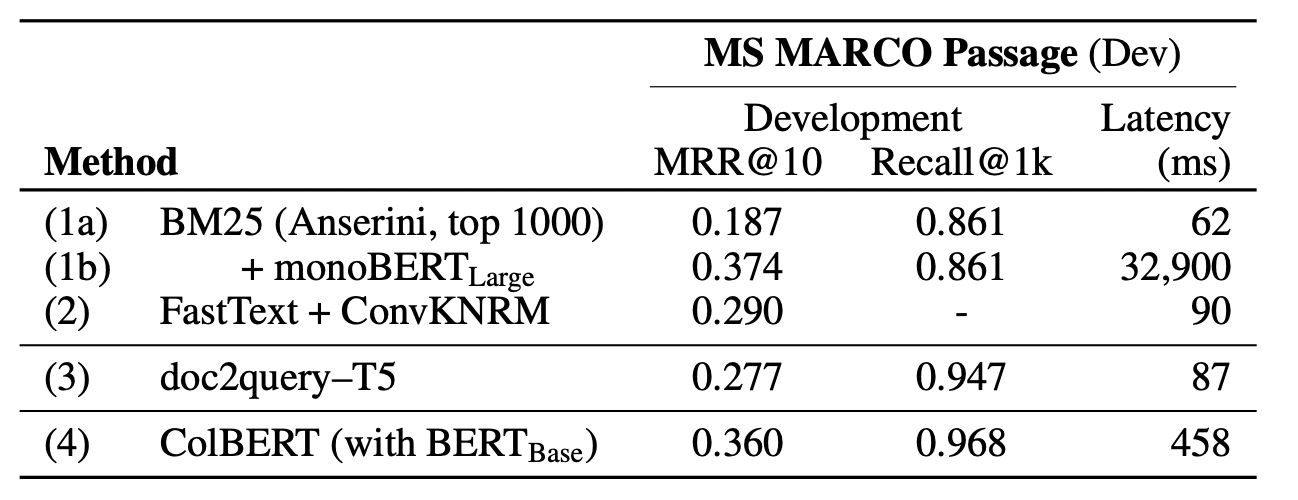
Colbert performs only slightly worse than monoBERT but is 2 orders of magnitude faster; however, it is still an order of magnitude slower than BM25.

So what's the catch? The index is orders of magnitude larger than that of BM25 to get the performance boost compared to monoBERT, the index needs to fit in memory to be searched efficiently.

Acknowledgements

These notes and tables are largely based on Pretrained Transformers for Text Ranking: BERT and Beyond.